Buyer's Guide to Redshift Architecture, Pricing, and Performance
Amazon Redshift is one of the fastest growing and most popular cloud services from Amazon Web Services. Redshift is a fully-managed, analytical data warehouse that can handle Petabyte-scale data, and enable analysts to query it in seconds.
The main advantage of Redshift over traditional data warehouses is that it has no upfront costs, does not require setup and maintenance, and is infinitely scalable using Amazon’s cloud infrastructure. You can scale Redshift on demand, by adding more nodes to a Redshift cluster, or by creating more Redshift clusters, to support more data or faster queries.
For more details, see our page about data warehouse architecture in this guide.
Want to quickly understand how Redshift works and what it can do for you?
In this article we’ll cover:
- Redshift architecture and a description of its main components
- Redshift cost and performance
- Redshift capabilities and features
- Taking a managed data warehouse to the next level
Redshift Architecture and Key Components
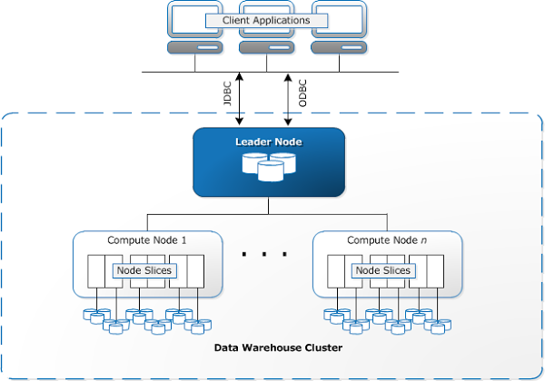 Source: AWS Documentation
Redshift Architecture in Brief
- Redshift supports client applications, such as BI, ETL tools or external databases, and provides several ways for those clients to connect to Redshift.
- Within Redshift, users can create one or more clusters. Each cluster can host multiple databases. Most projects require only one Redshift cluster; additional clusters can be added for resilience purposes (see this post by AWS on the subject).
- Each cluster comprises a leader node, which coordinates analytical queries, and compute nodes, which execute the queries. A high-speed internal network connects all the cluster nodes together to ensure high-speed communication.
- Each node is divided into slices, which are effectively shards of the data. Within each node are one or more databases based on PostgreSQL. The Redshift implementation is different from a regular PostgreSQL implementation, which stores user data.
Client Applications
Redshift integrates with a large number of applications, including BI and analytics tools, which enable analysts to work with the data in Redshift. Redshift also works with Extract, Transform, and Load (ETL) tools that help load data into Redshift, prepare it, and transform it into the desired state.
Because Redshift is based on PostgreSQL, most SQL applications can work with Redshift. However, there are important differences between the regular PostgreSQL version and the version used within Redshift.
Connection Methods
Client applications can communicate with Redshift using standard open-source PostgreSQL JDBC and ODBC drivers.
Since 2015, Amazon provides custom ODBC and JDBC drivers optimized for Redshift, which can provide a performance gain of up to 35% compared to the open-source drivers. Commercial vendors including Informatica, Microstrategy, Pentaho, Qlik, SAS and Tableau have already implemented these custom drivers in their solutions.
Clusters, Leader and Computer Nodes
When a user sets up an Amazon Redshift data warehouse, their core unit of operations is a cluster. A Redshift cluster is composed of one or more Compute Nodes. If more than one Compute Nodes exist, Amazon automatically launches a Leader Node which is not billed to the user. Client applications communicate only with the Leader Node. The Compute Nodes under the Leader Node are transparent to the user.
The Redshift Leader Node and Compute Nodes work as follows:
-
The Leader Node receives queries and commands from client programs.
-
When clients perform a query, the Leader Node is responsible for parsing the query and building an optimal execution plan for it to run on the Compute Nodes, based on the portion of data stored on each node.
-
Based on the execution plan, the Leader Node creates compiled code and distributes it to the Compute Nodes for processing. Finally, the Leader Node receives and aggregates the results, and returns the results to the client application.
A few additional details about Leader and Compute nodes:
- The Leader Node only distributes SQL queries to the compute nodes if the query references user-created tables or system tables. In Redshift, these are tables with an STLor STV prefix, or system views with an SVL or SVV prefix.
- Each Compute Node has dedicated CPU, memory, and attached disk storage. There are two node types: dense storage nodes and dense compute nodes. Storage for each node can range from 160 GB to 16 TB— the largest storage option enables storing Petabyte-scale data.
- As workload grows, you can increase computing capacity and storage capacity by adding nodes to the cluster, or upgrading the node type.
- Amazon Redshift uses high-bandwidth network connections, close physical proximity, and custom communication protocols to provide private, high-speed network communication between the nodes of the cluster.
- The compute nodes run on a separate, isolated network that client applications never access directly, which also has security benefits.
For more details, see our page about Redshift cluster architecture in this guide.
Node Slices
In Redshift, each Compute Node is partitioned into slices, and each slice receives part of the memory and disk space. The Leader Node distributes data to the slices, and allocates parts of a user query or other database operation to the slices. Slices work in parallel to perform the operations.
The number of slices per node depends on the node size of the cluster—see the number of slices for different node types.
Within the node, Redshift can decide automatically how to distribute data between the slices, or you can specify one column as the distribution key. When you execute a query, the query optimizer on the Leader Node redistributes the data on the Compute Nodes as needed, in order to perform any joins and aggregations.
The goal of defining a table distribution key is to minimize the impact of the redistribution step, by locating the data where it needs to be before the query is executed.
Amazon suggests three “styles” for choosing a distribution key, to help Redshift execute queries more efficiently.
- Distribute fact table and one dimension table on common columns: Your fact table can have only one distribution key. Choose one dimension to collocate based on how frequently it is joined and the size of the joining rows.
- Choose a column with high cardinality in the filtered result set: For example, if you distribute a sales table on a date column, you the result is an even data distribution (unless sales are seasonal). However, if queries are typically filtered for a narrow date period, the required rows are located on only a small set of slices, and queries run slower.
- Change some dimension tables to use ALL distribution: If a dimension table cannot be collocated with the fact table or other joining tables, you can improve query performance by distributing the entire table to all of the nodes. However there is a major drawback - using ALL distribution multiplies storage space requirements and increases load times and maintenance operations.
Databases
User data is stored on the Compute Nodes, in one or more databases. Client applications do not access the databases directly, because the SQL clients communicate only with the Leader Node, which coordinates query execution with the Compute Nodes.
Amazon Redshift is essentially an RDBMS system, and supports online transaction processing (OLTP) functions such as inserting and deleting data. However, unlike regular RDBMS databases, Redshift is optimized for high-performance analysis and reporting of very large datasets.
Redshift is based on PostgreSQL 8.0.2. Amazon Redshift and PostgreSQL have some important differences that should be taken into account.
Redshift Cost and Performance
The cost of storage and processing, and the speed at which you can execute large queries, are probably the most important criteria for selecting a data warehouse. The data below is based on Panoply’s in-depth Redshift vs. BigQuery paper, which you are invited to read in more detail.
Cost
Redshift’s pricing model is based on cluster nodes. You need to choose between Dense Compute and Dense Storage nodes. There are currently two options for each, ranging from 0.16-16 GB of storage, 2-36 virtual CPUs, and 15-244 GB of RAM.
Prices vary slightly based on Amazon data center; as of 2017 they range from approx. $0.25 per hour for the smaller Dense Computer node, to approx. $6.8 per hour for the larger Dense Storage node (see Amazon’s pricing page for the latest pricing). If you order a Reserved Instance, there are discounts of up to 75% compared to the per-hour pricing.
A common rule of thumb for Amazon Redshift pricing is that the cost of a Redshift data warehouse is under $1000/TB/Year for Dense Storage nodes, which scale to over a petabyte of compressed data. Dense Compute nodes scale up to hundreds of compressed terabytes for $5,500/TB/Year (3 Year Partial Upfront Reserved Instance pricing).
* This information is based on the Amazon Redshift Pricing Page.
Redshift Features and Capabilities
Below we briefly describe the following key Redshift features:
Columnar Storage and MPP Processing
Columnar Storage and MPP Processing are the basic Redshift features that enable high performance analytical query processing.
Analytical queries are typically run on multiple rows of data within the same column, as opposed to OLTP queries, which tend to process data row-by-row. In a traditional database, to sum up invoice amounts across a billion database rows, you need to scan the entire data set. Because Redshift uses a columnar structure, it can directly read the column representing the invoice amounts, and sum them up very quickly. Columnar storage not only improves query speed, but save on I/O operations, and can reduce storage size required for the same data sets.
As described in the architecture section above, Redshift employs a Massively Parallel Processing (MPP) architecture that distributes SQL operations across data slices within multiple cluster nodes, resulting in very high query performance. Redshift is also able to reorganize the data on the nodes before running a query, which dramatically boosts performance.
For more details, see our page on Redshift Columnar Storage in this guide.
Compression
Redshift automatically compresses all data you load into it, and decompresses it during query execution. Compression conserves storage space and reduces the size of data that is read from storage, which reduces the amount of disk I/O, and therefore improves query performance.
In Redshift, Compression is a column-level operation. There are several options for compressing data based on the columnar structure of the data.
Management and Security
Redshift is a managed service from Amazon, meaning that most of the ongoing tasks and concerns in a traditional data warehouse are taken care of:
- Managed infrastructure: Amazon provides the physical hardware, configuration, networking, and ongoing maintenance to ensure the data warehouse runs and performs optimally. However, Redshift does require users to perform maintenance via the VACUUM feature. VACUUM is a command that remove rows that are no longer needed in the database, and re-sorts the data. Amazon also doesn’t take responsibility for optimizing performance on the nodes for users’ specific queries or workloads.
- Backup and failover: Data stored in Redshift is replicated in all cluster nodes and is automatically backed up. Snapshots are maintained in S3 and can be restored. Amazon monitors the health of the Redshift cluster, re-replicates data from failed drives and replaces nodes as necessary. For additional resilience, Amazon enables running on multiple Availability Zones, where copies of the Redshift cluster run on more than one Amazon data center.
- Encryption: You can choose to encrypt all data on Redshift when creating data tables. You can also set cluster encryption when launching a cluster, to encrypt data in all user-created tables within the cluster.
- SSL: It is possible to encrypt connections between clients and Redshift. Redshift uses hardware-accelerated SSL while loading data from Amazon S3 or DynamoDB, during import, export, and backup.
- Virtual Private Cloud (VPC): Redshift leverages Amazon’s VPC infrastructure, enabling you to protect access to your cluster by using a private network environment within the Amazon data center.
See Redshift’s security overview for more details and options.
Data Types
Redshift supports a wide range of classic data types, listed below:
| Data Type | Description |
|---|---|
| SMALLINT | Signed two-byte integer |
| INTEGER | Signed four-byte integer |
| BIGINT | Signed eight-byte integer |
| DECIMAL | Exact numeric of selectable precision |
| REAL | Single precision floating-point number |
| DOUBLE PRECISION | Double precision floating-point number |
| BOOLEAN | Logical Boolean (true/false) |
| CHAR | Fixed-length character string |
| VARCHAR | Variable-length character string with a user-defined limit |
| DATE | Calendar date (year, month, day) |
| TIMESTAMP | Date and time (without time zone) |
| TIMESTAMPTZ | Date and time (with time zone) |
The DECIMAL (also called NUMERIC) data type stores values with user-defined precision. Precision is important for exact numeric operations, such as in financial operations.
For more details see our extensive blog post on challenges and best practices of Redshift data types.
Updates and Upserts
Amazon does advertise Redshift as a fully-featured RDBMS, but because it is highly optimized for analytical queries, updates and upserts are not trivial operations.
Redshift supports UPDATE and DELETE SQL commands internally, but does not provide a single merge or upsert command to update a table from a single data source. You can perform a merge operation by loading the updated data to a staging table, and then update the target table from the staging table. For more details, see the Redshift documentation page on updating and inserting.
Performing a large number of updates results in performance degradation over time, until a VACUUM operation is manually triggered. A VACUUM operation reclaims space and re-sorts rows in either a specified table or all tables in the current database. Running a VACUUM command without the necessary table privileges (table owner or superuser) has no effect.
Redshift Challenges
Amazon Redshift is a powerful service that has taken data warehouse technology to the next level. However, users still experience complexity when setting up Redshift:
- Loading data to Redshift is non-trivial. For large-scale data pipelines, loading data to Redshift requires setting up, testing and maintaining an ETL process. This is not taken care of in the Redshift offering.
- Updates, upserts and deletions can be tricky in Redshift and must be done carefully to prevent degradation in query performance.
- Semi-structured data is difficult to deal with, and needs to be normalized into a relational database format, which requires automation for large data streams.
- Nested structures are not supported in Redshift. You need to flatten nested tables into a format Redshift can understand.
- Optimizing your cluster: There are many options for setting up a Redshift cluster. Different workloads, data sets, or even different types of queries might require a different cluster setup. To stay optimal, you need to continually revisit your cluster setup and tweak the number and type of nodes.
- Query optimization: User queries may not follow best practices, and consequently take much longer to run. You may find yourself working with users or automated client applications to optimize queries, so that Redshift can perform as expected.
- Backup and recovery: While Amazon provides numerous options for backing up your data warehouse, these options are not trivial to set up and require monitoring and close attention.
Panoply is a cloud data platform that makes it easy to sync and store your data. With code-free ETL and a data warehouse built in, you can go from raw data to analysis-ready tables in a flash…and without the costly overhead that comes with traditional data infrastructure projects.
Learn more about Panoply.