Data Warehouse Architecture: Traditional vs. Cloud Models, Explained

Quick answer:

Traditional data warehouse architecture uses three tiers: a database server, an OLAP server and client tools for analysis. These run on hardware you own, sized for peak load.

Cloud warehouses such as Redshift, BigQuery and Snowflake separate storage from compute, scale each on demand and bill for use. Lakehouses add open table formats over files in cloud storage, letting you apply warehouse-style querying to data without moving it all into a separate warehouse.

A data warehouse is an electronic system that gathers data from a wide range of sources within a company and uses the data to support management decision-making.

Companies are increasingly moving towards cloud-based data warehouses instead of traditional on-premise systems. Cloud-based data warehouses differ from traditional warehouses in the following ways:

• There is no need to purchase physical hardware.
• It’s quicker and cheaper to set up and scale cloud data warehouses.
• Cloud-based data warehouse architectures separate storage from compute, so each can scale and be billed on its own, and they combine massively parallel processing (MPP) with columnar storage and compression to run complex analytical queries quickly.

The rest of this article covers traditional data warehouse architecture and introduces some architectural ideas and concepts used by the most popular cloud-based data warehouse services: Amazon Redshift, Google BigQuery and Snowflake, plus the lakehouse platforms that now compete with them.

For more details, see our page about data warehouse concepts in this guide.

Traditional Data Warehouse Architecture

The following concepts highlight some of the established ideas and design principles used for building traditional data warehouses.

Three-Tier Architecture

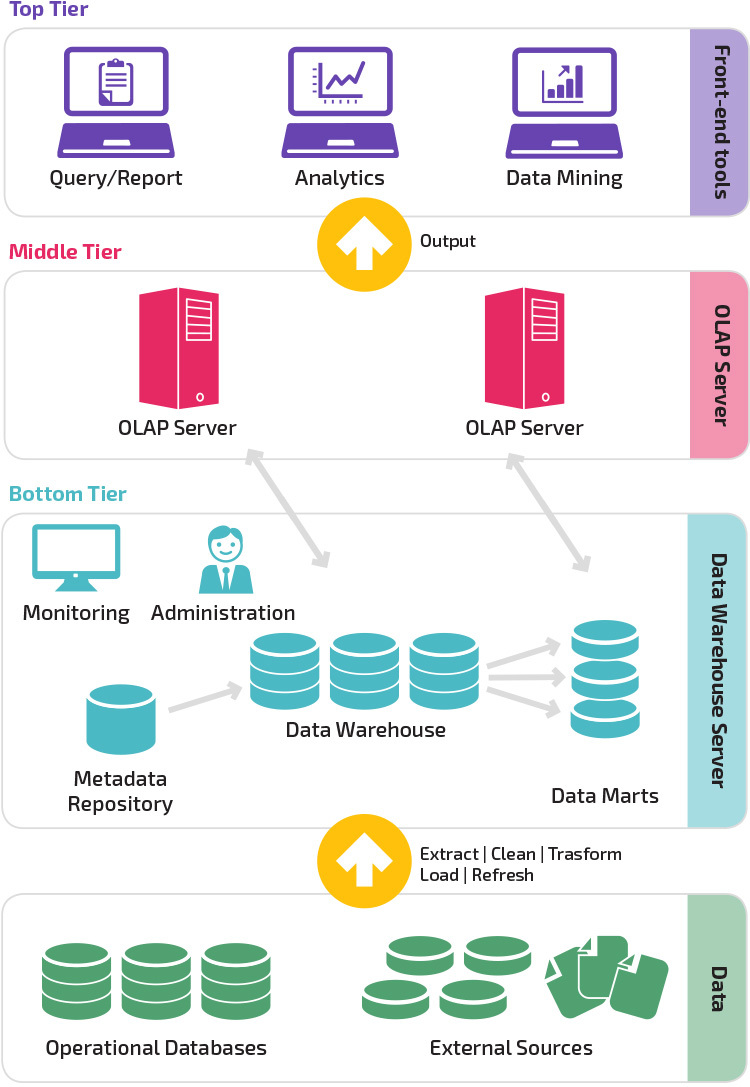
Traditional data warehouse architecture employs a three-tier structure composed of the following tiers.

• Bottom tier: This tier contains the database server used to extract data from many different sources, such as from transactional databases used for front-end applications.
• Middle tier: The middle tier houses an OLAP server, which transforms the data into a structure better suited for analysis and complex querying. The OLAP server can work in two ways: either as an extended relational database management system that maps the operations on multidimensional data to standard relational operations (Relational OLAP), or using a multidimensional OLAP model that directly implements the multidimensional data and operations.
• Top tier: The top tier is the client layer. This tier holds the tools used for high-level data analysis, querying, reporting, and data mining.

Kimball vs. Inmon

Two pioneers of data warehousing named Bill Inmon and Ralph Kimball had different approaches to data warehouse design.

Ralph Kimball’s approach stressed the importance of data marts, which are repositories of data belonging to particular lines of business. The data warehouse is simply a combination of different data marts that facilitates reporting and analysis. The Kimball data warehouse design uses a “bottom-up” approach.

Bill Inmon regarded the data warehouse as the centralized repository for all enterprise data. In this approach, an organization first creates a normalized data warehouse model. Dimensional data marts are then created based on the warehouse model. This is known as a top-down approach to data warehousing.

Most teams today blend both approaches, loading a central cloud warehouse and modelling Kimball-style dimensional marts on top. The choice matters less than agreeing on one place for shared definitions, such as the metrics that sales and finance both report.

Data Warehouse Models

In a traditional architecture there are three common data warehouse models: virtual warehouse, data mart, and enterprise data warehouse:

• A virtual data warehouse is a set of separate databases, which can be queried together, so a user can effectively access all the data as if it was stored in one data warehouse.
• A data mart model is used for business-line specific reporting and analysis. In this data warehouse model, data is aggregated from a range of source systems relevant to a specific business area, such as sales or finance.
• An enterprise data warehouse model prescribes that the data warehouse contain aggregated data that spans the entire organization. This model sees the data warehouse as the heart of the enterprise’s information system, with integrated data from all business units.

Star Schema vs. Snowflake Schema

The star schema and snowflake schema are two ways to structure a data warehouse.

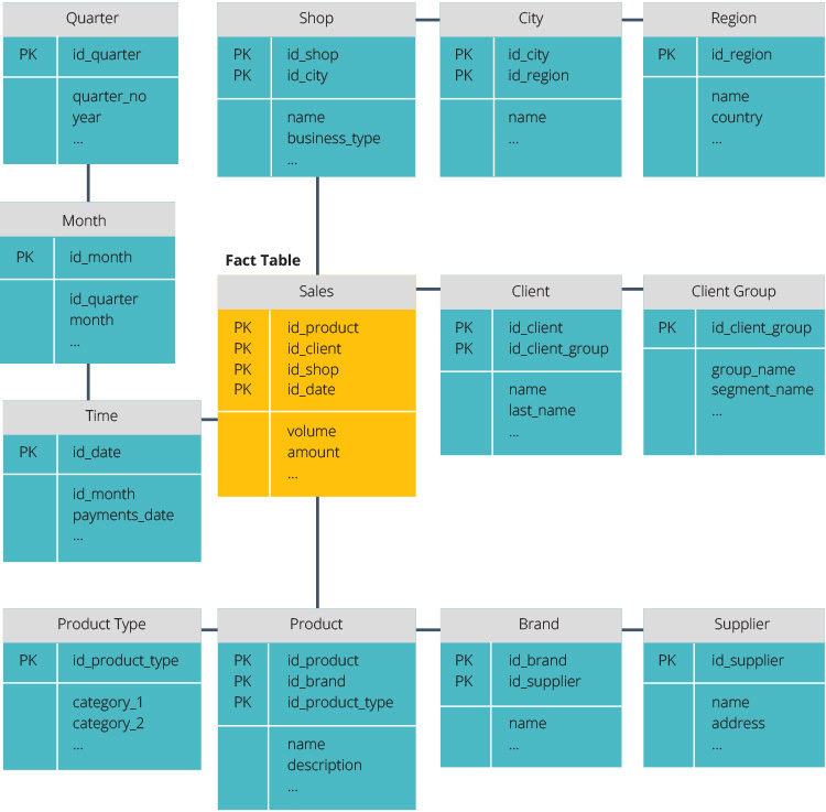
The star schema has a centralized data repository, stored in a fact table. The fact table sits at the center and links to a series of denormalized dimension tables. The fact table holds the measurements of a business process at a declared grain, usually one row per event such as an order line, while the dimension tables describe the stored data.

Denormalized designs are less complex because the data is grouped. The fact table uses only one link to join to each dimension table. The star schema’s simpler design makes it much easier to write complex queries.

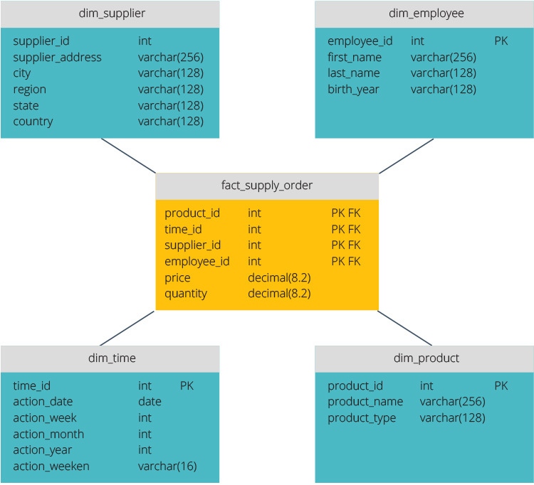
The snowflake schema is different because it normalizes the data. Normalization means efficiently organizing the data so that all data dependencies are defined, and each table contains minimal redundancies. Single dimension tables thus branch out into separate dimension tables.

The snowflake schema uses less disk space and better preserves data integrity. The main disadvantage is the complexity of queries required to access data: each query must dig deep to get to the relevant data because there are multiple joins.

In cloud warehouses, storage is cheap compared with the compute cost of repeated joins at query time, so star schemas and wide denormalized tables are common. Google says BigQuery performs best when data is denormalized and suggests nested and repeated columns to keep relationships without joins.

ETL vs. ELT

ETL and ELT are two different methods of loading data into a warehouse.

Extract, Transform, Load (ETL) first extracts the data from a pool of data sources, which are typically transactional databases. The data is held in a temporary staging database. Transformation operations are then performed, to structure and convert the data into a suitable form for the target data warehouse system. The structured data is then loaded into the warehouse, ready for analysis.

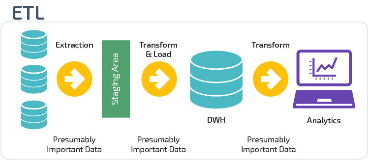
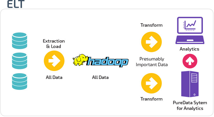
With Extract Load Transform (ELT), data is loaded right after being extracted from the source data pools. There is no separate staging database: raw data lands in the warehouse itself, often in a raw or staging schema, and is transformed inside the data warehouse system for use with business intelligence tools and analytics.

ELT is now the default pattern for cloud warehouses. For cloud ELT, Fivetran or Airbyte loads raw tables; dbt transforms them with SQL. Compare ingestion and transformation options in ETL tools.

Organizational Maturity

The structure of an organization’s data warehouse also depends on its current situation and needs.

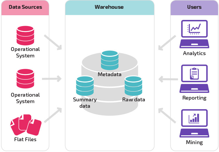
The basic structure lets end users of the warehouse directly access summary data derived from source systems and perform analysis, reporting, and mining on that data. This structure is useful for when data sources derive from the same types of database systems.

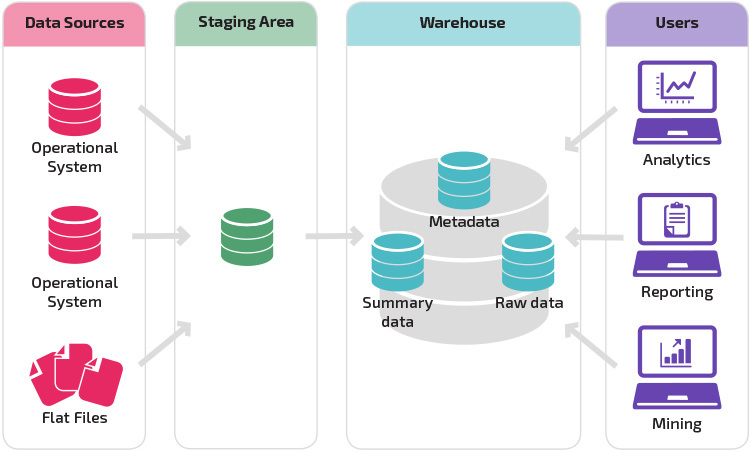
A warehouse with a staging area is the next logical step in an organization with disparate data sources with many different types and formats of data. The staging area converts the data into a summarized structured format that is easier to query with analysis and reporting tools.

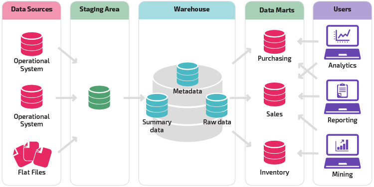
A variation on the staging structure is the addition of data marts to the data warehouse. The data marts store summarized data for a particular line of business, making that data easily accessible for specific forms of analysis. For example, adding data marts can allow a financial analyst to more easily perform detailed queries on sales data, to make predictions about customer behavior. Data marts make analysis easier by tailoring data specifically to meet the needs of the end user.

New Data Warehouse Architectures

In recent years, data warehouses have moved to the cloud. The new cloud-based data warehouses do not adhere to the traditional architecture; each data warehouse offering has a unique architecture.

This section summarizes the architectures used by three of the most popular cloud-based warehouses: Amazon Redshift, Google BigQuery and Snowflake.

What the Cloud Models Share

Cloud models separate storage from compute so each scales independently. You rent capacity instead of buying hardware sized for peak load; the vendor handles patching, upgrades and physical infrastructure. On-premises appliances also used MPP and columnar storage. Cloud elasticity lets you change query capacity without replacing servers or expanding storage.

Amazon Redshift

Amazon Redshift is a cloud-based representation of a traditional data warehouse.

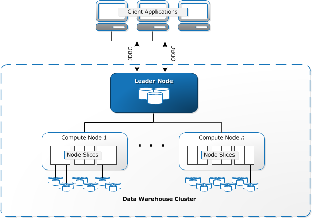
Provisioned Redshift clusters contain a collection of one or more nodes. A leader node compiles queries and transfers them to compute nodes, which execute the queries. On current RA3 and RG nodes, data lives in Redshift Managed Storage backed by Amazon S3, so compute and storage scale and are billed separately; AWS has deprecated the older DC2 nodes, which kept all data on local disks. Redshift Serverless removes the cluster altogether: it provisions capacity automatically and you pay only while the warehouse is in use.

Each compute node is partitioned into slices, and each slice gets a portion of the node’s memory and disk space and processes a portion of the workload. Redshift uses a columnar storage, meaning each block of data contains values from a single column across a number of rows, instead of a single row with values from multiple columns.

Source: AWS Documentation

Redshift uses an MPP architecture, breaking up large data sets into chunks which are assigned to slices within each node. Queries perform faster because the compute nodes process queries in each slice simultaneously. The Leader Node aggregates the results and returns them to the client application.

Client applications, such as BI and analytics tools, can directly connect to Redshift using the Amazon Redshift JDBC, ODBC and Python drivers; AWS does not support generic PostgreSQL drivers for Redshift. Analysts can thus perform their tasks directly on the Redshift data.

Redshift is no longer limited to structured data: the SUPER type stores semi-structured and nested data such as JSON, queried with PartiQL. It is possible to load data to Redshift with the COPY command from Amazon S3 and DynamoDB or from remote hosts over SSH, through streaming ingestion from Kinesis Data Streams or Amazon MSK, and through zero-ETL integrations with Aurora, RDS, DynamoDB and applications such as Salesforce and SAP.

For more detail on query processing and provisioning, see the chapters on Redshift architecture and Redshift clusters.

Google BigQuery

BigQuery’s architecture is serverless, meaning Google dynamically manages the allocation of machine resources. All resource management decisions are, therefore, hidden from the user.

BigQuery lets clients load data from Google Cloud Storage and other readable data sources. The alternative option is to stream data, which allows developers to add data to the data warehouse in real-time, row-by-row, as it becomes available. For new streaming pipelines, Google recommends the Storage Write API.

BigQuery uses a query execution engine named Dremel, which turns each SQL query into an execution tree. Dremel uses massively parallel querying to scan data in the underlying Colossus distributed file system. Google’s Jupiter network moves data between the stages of a query, and Borg, Google’s cluster manager, allocates the machines.

Dremel uses a columnar data structure, similar to Redshift. In the tree, leaves called slots read data from Colossus and do the computation, and branches called mixers aggregate the results.

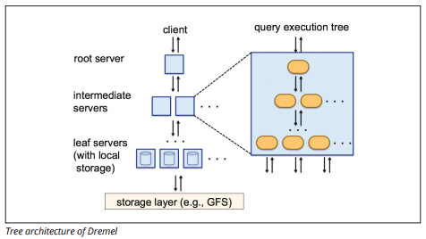
Image source: Google, BigQuery technical white paper

Simple SQL commands are used to perform queries on data. Because storage and compute are separate, you pay either for the bytes each query scans (on-demand pricing) or for reserved slot capacity through BigQuery editions.

See the BigQuery architecture chapter for a deeper explanation of how its storage and query processing components work together.

Snowflake

Snowflake runs on AWS, Azure and Google Cloud, not on premises or in a private cloud. Its hybrid shared-disk and shared-nothing architecture combines shared storage with independent compute clusters.

Snowflake has three layers: database storage, query processing and cloud services. Query processing runs in virtual warehouses, each an independent compute cluster, so a loading job and a BI dashboard can use separate warehouses without competing for the same compute resources. The cloud services layer handles authentication, metadata management and query optimization, separate from the virtual warehouses that execute your workloads.

Data is stored in columnar, compressed micro-partitions, each containing 50 MB to 500 MB of uncompressed data. VARIANT columns hold semi-structured data such as JSON without requiring you to flatten it before loading. Time Travel retains changed or deleted data for 1 day by default, with retention of up to 90 days for permanent tables on Enterprise Edition and higher.

Traditional vs. Cloud Data Warehouse Architecture at a Glance

Compare who owns the infrastructure, how capacity grows and what you pay for before choosing a model.

	Traditional (on-premises)	Cloud data warehouse
Hardware	Servers or appliances you buy and run	None, the vendor runs it
Storage and compute	Tied together on the same machines	Separated, each scales on its own
Scaling	Buy and install more hardware, sized for peak	Resize, add clusters or let a serverless service scale
Cost model	Up-front capital cost plus licences	Pay for compute time or data scanned, plus storage
Data types	Structured, relational	Structured plus semi-structured and nested data such as JSON
Loading pattern	ETL with a separate staging database	Mostly ELT, transformations run inside the warehouse
Maintenance	Your team patches, tunes and backs up	Vendor handles hardware and upgrades, time travel covers many recoveries

The cloud column covers different billing models. Compare Redshift, BigQuery, Snowflake, Databricks and Microsoft Fabric on costs for your actual workload, not query speed alone. Use the warehouse pricing playbook to compare cost models and the data warehouses chapter to narrow your options before committing to a platform.

Beyond Cloud Data Warehouses

Cloud-based data warehouses are a big step forward from traditional architectures. However, users still face several challenges when setting them up:

• Loading data to cloud data warehouses is non-trivial, and for large-scale data pipelines, it requires setting up, testing, and maintaining an ETL or ELT process. This part of the process is typically done with third-party tools such as Fivetran and Airbyte, or with built-in options such as Redshift zero-ETL.
• Updates, upserts, and deletions can be tricky and must be done carefully to prevent degradation in query performance.
• Semi-structured data no longer has to be normalized before loading: Redshift SUPER, Snowflake VARIANT and BigQuery nested columns store it directly, although frequently queried fields still run faster as typed columns or materialized views.
• Nested structures are supported natively by BigQuery (STRUCT and ARRAY), Snowflake (OBJECT and ARRAY) and Redshift (SUPER), so flattening nested tables is now a modelling choice rather than a requirement.
• Backup and recovery: while data warehouse vendors provide numerous options for backing up your data, they are not trivial to set up and require monitoring and close attention.

Lakehouses and Open Table Formats

Databricks defines a data lakehouse as a data management system combining the benefits of data lakes and data warehouses. Delta Lake adds a transaction log to Parquet files for ACID transactions, schema enforcement and table history. Databricks SQL warehouses run warehouse-style SQL on these tables, and Databricks recommends the serverless type where it is available. Apache Iceberg is another open table format: Snowflake, BigQuery and Redshift can query Iceberg tables whose files sit in cloud storage you own, allowing a shared copy to serve several engines.

Microsoft Fabric Data Warehouse stores Delta tables in OneLake, with independently scalable storage and compute; Azure Synapse dedicated SQL pools remain available. Many lakehouses organize data in medallion layers: bronze holds raw data as it arrives, silver holds cleaned, deduplicated and joined data, and gold holds aggregates for BI and ML. These lake-file layers mirror the traditional staging area and data marts above. See data warehouse vs. data lake for the broader distinction.

Choosing an Architecture Today

Start with the warehouse that matches the cloud you already use: Redshift on AWS, BigQuery on Google Cloud or Fabric on Azure. A multicloud option such as Snowflake lets you use a similar architecture across supported cloud providers. Load with a managed ELT tool, transform with dbt, and keep a star schema for the BI layer so reporting queries stay understandable.

Before relying on built-in recovery, check the retention windows against how quickly your team detects mistakes. BigQuery time travel defaults to 7 days and is configurable from 2 to 7 days; Snowflake Time Travel defaults to 1 day. Consider a lakehouse when most data already sits in files or several engines must share it.

Common questions

What are the three tiers of data warehouse architecture?

The bottom tier holds the database server, the middle tier holds the OLAP server, and the top tier holds client tools for querying, reporting and analysis. The OLAP server can use relational OLAP (ROLAP) or multidimensional OLAP (MOLAP). See Three-Tier Architecture above for the full breakdown.

What is the difference between a traditional and a cloud data warehouse?

A traditional warehouse runs on hardware you own, usually with storage and compute coupled together. A cloud warehouse rents vendor-managed infrastructure and separates storage from compute so each can scale independently. You pay for usage or allocated capacity instead of buying servers sized for peak demand. Serverless options automate capacity provisioning.

Is a star schema or a snowflake schema better?

A star schema is usually the better starting point for BI and cloud warehouses because it needs fewer joins and makes queries simpler. A snowflake schema reduces redundancy and preserves data integrity, but adds joins. BigQuery also supports nested and repeated columns as an alternative to heavily normalized tables.

What is the difference between a data warehouse, a data lake and a lakehouse?

A data warehouse organizes data into modeled tables for SQL analysis, while a data lake holds raw files of any type. A lakehouse adds warehouse features to lake files through open table formats such as Delta Lake or Iceberg, which add ACID transactions and table history to those files. See Lakehouses and Open Table Formats above for examples.

Can a cloud data warehouse store JSON?

Yes. Redshift stores JSON in SUPER columns and queries it with PartiQL, Snowflake uses VARIANT, and BigQuery supports nested and repeated columns for structured representations of JSON data. You do not have to flatten every nested structure before loading. For frequent queries, typed columns or materialized views can improve performance.

Where to next

Review Data Warehouse Concepts for the underlying terminology and modeling concepts, or Database vs. Data Warehouse to distinguish operational storage from analytics. Continue to the next chapter, Data Mart vs. Data Warehouse, for business-specific reporting structures. When you are ready to plan ingestion, Full vs Incremental Loading explains how to move source data into the warehouse without reloading everything each time.