A Deep Dive Into Google BigQuery Architecture: How It Works

Google’s BigQuery is an enterprise-grade cloud-native data warehouse. BigQuery became generally available in 2011. Since inception, BigQuery has evolved into a fully-managed data warehouse which can run interactive and ad-hoc queries on datasets of petabyte-scale. In addition, BigQuery integrates with a variety of Google Cloud services and third-party tools.

BigQuery is serverless, or more precisely data warehouse as a service. There are no servers to manage or database software to install. BigQuery service manages underlying software as well as infrastructure including scalability and high-availability. Storage and compute are billed separately: on-demand queries are charged by data processed, while capacity-based pricing charges for slots over time.

Overall, you don’t need to know much about underlying BigQuery architecture or how this service operates under the hood. That’s the whole idea of BigQuery: you don’t need to manage the underlying infrastructure. To get started with BigQuery, you must be able to load or connect to your data, then write your queries using GoogleSQL.

Having said that, a good understanding of how Google BigQuery architecture works is useful when implementing various BigQuery best-practices including controlling costs, optimizing query performance, and optimizing storage. For instance, for best query performance, it is highly beneficial to understand how BigQuery allocates resources and the relationship between the number of slots and query performance.

High-level architecture

BigQuery is built on top of Dremel technology which has been in production internally in Google since 2006. The original Dremel paper described Google’s interactive ad-hoc query system for analysis of read-only nested data. It was published in 2010 and at the time of publication Google was running multiple instances of Dremel ranging from tens to thousands of nodes.

10,000 foot view

BigQuery’s architecture builds on Dremel. By incorporating columnar storage and the tree architecture of Dremel, BigQuery can distribute analytical work across many machines. But BigQuery is much more than Dremel. Dremel is the query execution engine for BigQuery.

BigQuery also uses Google’s infrastructure technologies, including Borg, Colossus, Capacitor, and Jupiter. As illustrated below, a BigQuery client (typically the Google Cloud console, bq command-line tool, or an API) interacts with the query engine through a client interface. Borg, Google’s large-scale cluster management system, allocates compute resources.

Dremel jobs read data from Colossus using the Jupiter network, perform SQL operations, and return results to the client. The original serving-tree model is covered in more detail in the execution section.

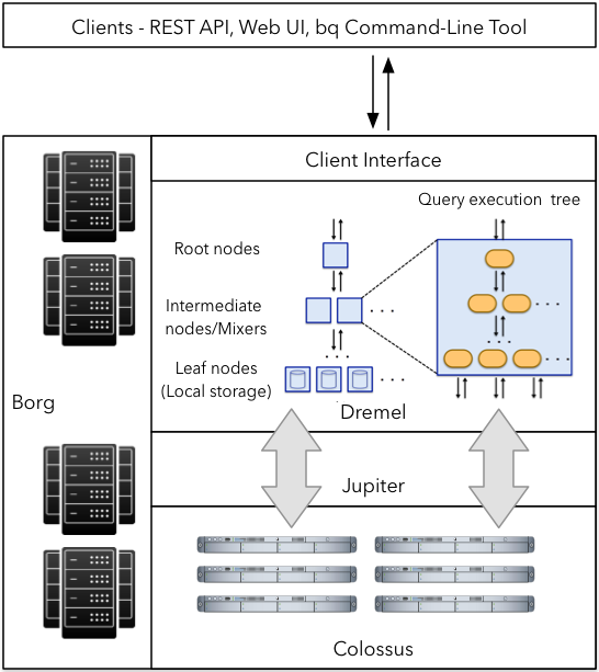
Figure-1: A high-level architecture for BigQuery service. The diagram shows the original Dremel model; modern query plans can use additional stages and data redistribution.

BigQuery architecture separates storage from compute and allows them to scale independently, a key requirement for an elastic data warehouse. Colossus provides distributed storage; Dremel performs query execution, with Borg managing the underlying compute resources.

Storage

Disk I/O is an important cost in large analytical queries. BigQuery stores data in a columnar format known as Capacitor. Each column is stored separately, which enables BigQuery to read the fields a query needs and compress similar values efficiently. In 2016, Capacitor replaced ColumnIO, the previous generation columnar storage format, and introduced the ability to perform operations directly on compressed data.

You can import your data into BigQuery storage via batch loads or streaming. During the import process, BigQuery encodes columns into Capacitor format and collects statistics used for query planning. The encoded data is written to Colossus, while BigQuery manages the physical file sizes and organization in the background.

For new streaming integrations, the Storage Write API (gRPC) supports continuously arriving data. Its default stream makes data immediately available for queries with at-least-once delivery. Application-created streams can provide exactly-once writes when the client manages stream offsets.

BigQuery uses Capacitor to store data in Colossus. Colossus is Google’s distributed file system and successor to GFS (Google File System). Colossus handles replication, recovery and distributed management.

BigQuery automatically stores copies of your data in two different zones within a single region. Cross-region replication is a separate choice; selecting a multi-region location does not itself provide regional redundancy.

Capacitor and Colossus work together to support parallel reads: Colossus provides distributed storage, while Capacitor reduces the data that needs to be read and processed. You can influence how much data a query scans through partitioning and clustering. Filters on the partition column can skip partitions, and filters on clustering columns can skip storage blocks.

Native vs. external

So far we have discussed the storage for the native BigQuery table. BigQuery can also perform queries against external data sources without the need to import data into the native BigQuery tables. External tables can reference Cloud Storage, Bigtable, or Google Drive. BigLake tables extend access controls to supported external stores, including options for Amazon S3 and Azure Blob Storage.

External tables and federated queries are related but different. An external table points to data stored outside BigQuery. A federated query can use EXTERNAL_QUERY to run SQL in a supported database, such as Cloud SQL, AlloyDB, or Spanner, and bring the results back into BigQuery.

Performance depends on the source, data format, and query. For repeated analytical workloads, compare native-table performance with the cost and freshness requirements of keeping the data in place.

Compute

BigQuery takes advantage of Borg for data processing. Borg runs Dremel jobs and assigns compute capacity across clusters of machines. In addition to assigning compute capacity for Dremel jobs, Borg handles fault-tolerance.

The capacity visible to you is measured in slots, virtual compute units used to execute queries. With on-demand pricing, queries use shared capacity and are billed by bytes processed. With capacity-based pricing, you create reservations in Standard, Enterprise, or Enterprise Plus editions.

Reservations can use baseline capacity, autoscaling, or both; eligible capacity commitments can reduce the price. The number of available slots affects concurrency and can affect query performance, but more slots do not make every query faster.

On-demand analysis starts at $6.25 per TiB processed, with the first 1 TiB per month free. Prices vary by location, and storage and some other operations have separate charges. For capacity pricing, compare slot-hour costs and utilization rather than multiplying scanned bytes by the on-demand rate. See BigQuery pricing for the rate in your region.

Network

Apart from disk I/O, big data workloads are often rate-limited by network throughput. Due to the separation between compute and storage layers, BigQuery requires a fast network to move data from storage into compute for running Dremel jobs. Google’s Jupiter network provides petabit-scale connectivity. This is shared infrastructure capacity, not a bandwidth allocation or query-runtime guarantee for an individual user.

Updating data

Columnar storage does not make BigQuery read-only. Data manipulation language statements support INSERT, UPDATE, DELETE, and MERGE, so you can modify existing tables as well as write query results into new ones. BigQuery is optimized for analytical workloads; these capabilities do not make it a substitute for a transactional database serving frequent individual-record updates.

Execution model

The original Dremel engine uses a multi-level serving tree for scaling out SQL queries. This tree architecture was designed to run on commodity hardware. Dremel uses a query dispatcher which not only provides fault tolerance but also schedules queries based on priorities and the load.

In current BigQuery, a query is represented as stages and execution steps. Stages exchange data through a distributed shuffle, and the plan can change while the query runs. The serving tree remains a useful way to understand partial aggregation, rather than a fixed blueprint for every query.

In a serving tree, a root server receives incoming queries from clients and routes the queries to the next level. The root server is responsible for returning query results to the client. Leaf nodes of the serving tree do the heavy lifting of reading the data from Colossus and performing filters and partial aggregation. To parallelize the query, each serving level (root and mixers) rewrites the query, and ultimately modified and partitioned queries reach the leaf nodes for execution.

During query rewrite, a few things happen. Firstly, the work is divided across horizontal pieces of the table (in the original Dremel paper these were called tablets). Secondly, some SQL clauses can be simplified before sending work to leaf nodes. In a Dremel tree, many leaf nodes can work in parallel.

Leaf nodes return results to mixers or intermediate nodes. Mixers perform aggregation of results returned by leaf nodes.

BigQuery automatically determines the parallelism needed for each query stage, depending on query size, complexity, and available capacity. With on-demand pricing, the published limits are 2,000 concurrent slots per project and 20,000 per organization. Slots are shared among queries in a project; transient bursts can exceed the limit, and capacity is subject to availability. These figures are not a guaranteed allocation to an individual query.

To help you understand how the Dremel engine works and how the serving tree executes an aggregation, let’s look into a simple query:

SELECT A, COUNT(B) FROM T GROUP BY A

When the root server receives this query, it translates it into a form which can be handled by the next level of the serving tree. It determines the pieces of table T that must be scanned, then combines the partial results. The expression below is conceptual pseudocode, not SQL you can run:

SELECT A, SUM(c) FROM (R1i UNION ALL ... R1n ) GROUP BY A

In this case, R1i through R1n represent partial results returned through the mixers, and c is a partial COUNT(B) for a value of A. Summing those counts produces the final result.

Next, mixers modify the incoming queries so that they can pass them to leaf nodes. Leaf nodes receive the work and read the required columns from Colossus. Each leaf computes partial results, which the mixers combine. The example illustrates the division of work rather than the exact low-level scan loop used by every current query.

Depending on the query, data may be shuffled between workers. For instance, GROUP BY and JOIN operations can require data to be redistributed. Some queries with operations like JOIN can run slowly unless you optimize them to reduce the shuffling. That’s why filtering or aggregating data early, where the query permits it, can reduce the data passed to later stages.

As BigQuery charges on-demand queries for data processed, we should avoid scanning too much or too frequently. There are many ways to do this. One is partitioning your tables by date and filtering on the partition column. If several queries reuse the same intermediate result, saving it in a temporary or destination table can avoid repeating the same work.

It may sound counter-intuitive, but the LIMIT clause does not reduce the amount of data scanned from a non-clustered table. Clustered tables are an exception: scanning can stop after enough blocks have been read to satisfy the limit. If you just need sample data for exploration, use the Preview option rather than paying for an unnecessary query scan.

BigQuery can adjust the execution plan and redistribute work while a query runs. To see where time and resources are spent, inspect the execution graph rather than estimating performance from the number of leaf nodes in the original diagram.

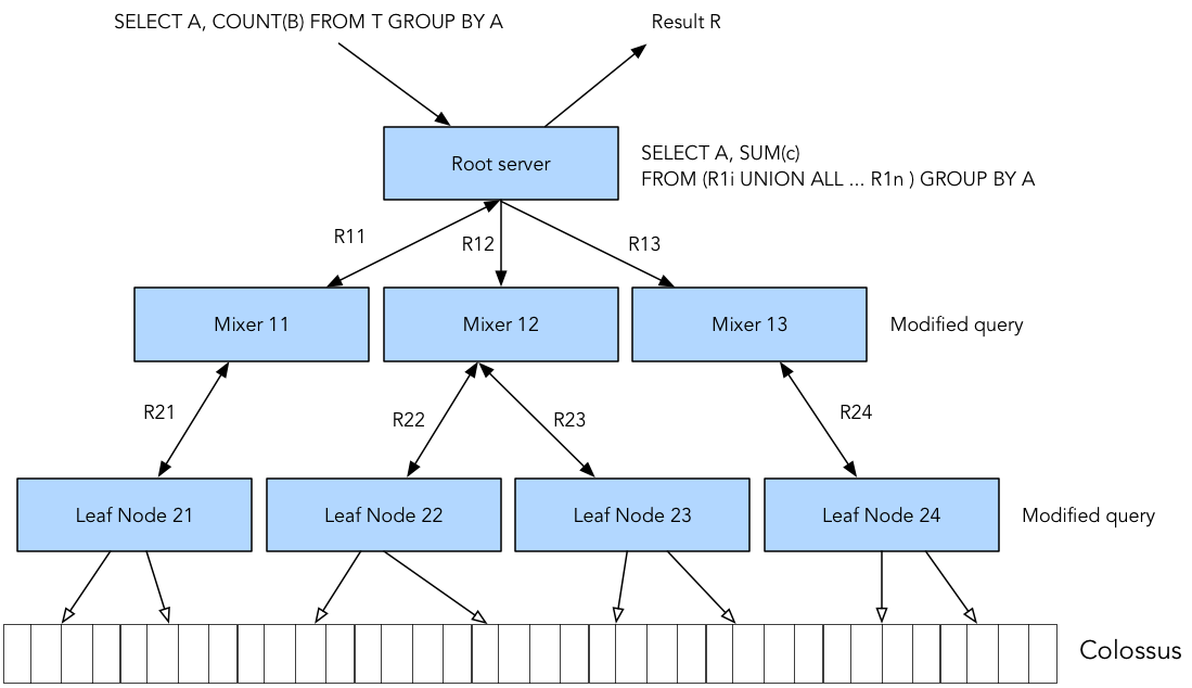
Figure-2: An example of the original Dremel serving tree.

Some mathematics

Now that we understand BigQuery architecture, let’s look at how column selection affects the amount of data a query processes. Say you are querying a table with 10 columns and 10 TiB of logical data. For this simplified example, assume each column accounts for 1 TiB, and there is no partition or cluster pruning.

A full scan using SELECT * reads all 10 TiB. A query that only needs two of those equally sized columns reads about 2 TiB, an 80% reduction in scanned data. Under on-demand pricing, that also reduces the scan-based query charge before free allowances or other billing adjustments. It does not imply an 80% reduction in execution time: joins, aggregation, shuffle, and available capacity also affect runtime.

We should query only the columns that we need, and that’s an important best-practice for any column-oriented database or data warehouse. Use a dry run or the query editor’s estimate to check bytes processed before executing an on-demand query.

Data model

BigQuery stores data as nested relations. The schema for a relation is represented by a tree. Nodes of the tree are attributes, and leaf attributes hold values. BigQuery data is stored in columns (leaf attributes).

In addition to compressed column values, every column also stores structure information to indicate how the values in a column are distributed throughout the tree using two parameters: definition and repetition levels. These parameters help to reconstruct the full or partial representation of the record by reading only requested columns.

Figure-3: An example of (a) tree schema and (b) an instance based on the schema.

To take advantage of nested and repeated fields offered by BigQuery, denormalize hierarchical data that you frequently query together. Denormalization localizes the necessary data to individual workers, which can reduce the network communication required for shuffling between slots. A well-designed star schema may gain little from further denormalization, so apply this to your query patterns rather than every relationship.

Query language

BigQuery supports GoogleSQL, formerly called Google Standard SQL, and legacy SQL, the original BigQuery dialect. GoogleSQL is ANSI-compliant and is the recommended choice for new queries and projects. Both dialects support user-defined functions (UDFs), but new development should use GoogleSQL rather than legacy syntax.

When denormalizing your data you can preserve some relationships by taking advantage of nested and repeated fields instead of completely flattening your data. In GoogleSQL, STRUCT represents nested fields and ARRAY represents repeated values. An ARRAY of STRUCT values can keep an order and its line items together; UNNEST exposes those elements as rows when the query needs them.

Alternatives

There are several alternatives to BigQuery, both open-source engines and managed cloud services. Running an engine such as Presto yourself means managing its infrastructure and operations. Amazon Athena provides serverless SQL analysis, commonly over data in Amazon S3; its engine version 3 incorporates developments from Trino and Presto.

The useful comparison is how each service fits your data, queries, and operating model. BigQuery combines managed storage with serverless query execution, while Athena is often used to query an existing S3 data lake. For a warehouse alternative, see our guide to Amazon Redshift architecture. Compare performance using your own workloads rather than treating early benchmarks as a permanent ranking.

Final thoughts

BigQuery is designed to query structured and semi-structured data using GoogleSQL. BigQuery is a cloud-based fully-managed service, so you do not provision the servers used for storage and query execution. It is well suited to interactive queries and OLAP/BI use cases. Google’s infrastructure technologies, including Borg, Colossus, and Jupiter, support that separation of storage and compute.

For practical performance improvements, start with the data your query reads: select the columns you need, use partition and clustering filters, and inspect the execution plan for expensive joins or shuffle. Choose on-demand or capacity-based compute around the workload you actually run.

References

Prices current as of October 2026.

In the directory

Warehouses, ETL and ELT tools in the directory

Snowflake, BigQuery, Redshift, Databricks, Fivetran, Airbyte and the rest, with pricing and what each one replaces.

Browse the tools